Preface🚀

Data engineering is a field that deals with turning raw data into useful and valuable information. It involves any activity that manipulates data into a format that can be used or digested by end users or applications to generate real-world value.

In today’s digital world, data engineering plays an ever-evolving part in building tools and technologies to make human life easier and more convenient to navigate through.

SQL 💾

SQL stands for Structured Query Language and is used for requesting data to be returned in a user-specified format from databases.

Before SQL🔙

To appreciate what SQL brings to the table, I thought we should delve into a bit of history as to how we used to store and retrieve data before it came into the picture.

Before SQL, data was stored & retrieved from:

• Paper files

• Flat files

• Hierarchical databases

• Network databases

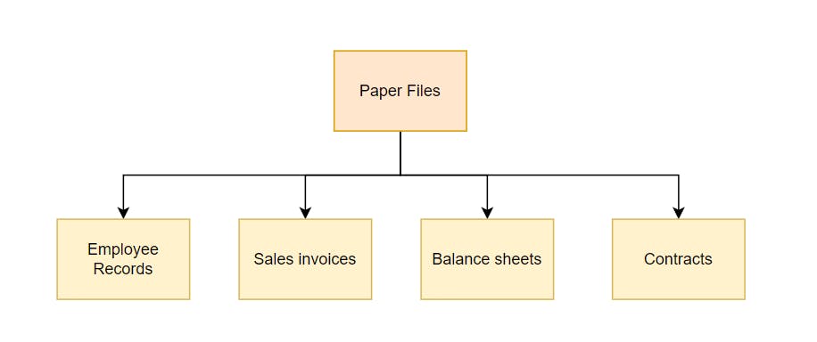
1. Paper files 🗃️🗄️

These represent any data stored physically, like records, documents and correspondences stored away in filing cabinets.

Key challenges with the paper file approach include:

• Manual retrieval 🚶🏽- Pulling data from physical stores takes time and physical energy

• Limited spaces 🏢- You are only restricted by the physical storage you had access to, and this is problematic as data grows over time

• Vulnerable to damages and disasters🧯- Paper can easily get torn, worn out or stained. Plus, they are at risk of unforeseen events such as theft, fire or even extreme weather conditions

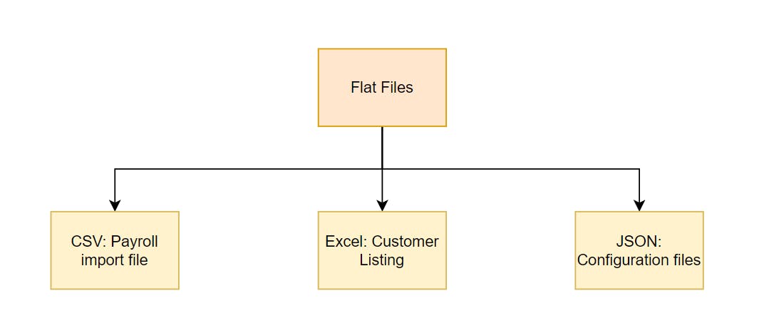
2. Flat Files 💻

This includes any data stored on computers in digital formats like Excel, CSVs, JSON etc. In today’s age, these are some of the most common data formats available and have addressed some of the data storage and retrieval challenges paper files came with.

Some of the problems with storing data in flat files over time include:

• No data relationships ❌🔗- Although it is possible to add unique identifiers to records in flat files, it is difficult to form complex relationships between tables with similar attributes due to the inability to enforce schemas and other useful constraints

• Scalability problems ⏫🐌- As data grows, so does the level of difficulty with retrieving data, just ask any team that uses Excel spreadsheets as their databases

• Redundant data 🔄📑- Another issue with growing data is having data duplicated across different areas - because there are no mechanisms to prevent them from entering, redundant data can appear in many places undetected

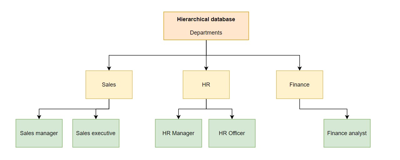
3. Hierarchical databases👪

Also referred to as hierarchical data models, these are databases that organise data in a way that resembles a tree, where there is one parent node (representing a single record, or the main record at the top) and child nodes (that represent the sub-records under the main record).

What made this appealing was how simple it was to use and retrieve data from it. By following the hierarchy of each node path, extracting data was relatively quick and straightforward compared to paper and flat file approaches. This was the start of efficient data storage and retrieval from databases.

But this approach had its downfalls:

• Data redundancy 🔄📑- Similar to the flat files, the same data may appear in multiple categories undetected, which lowers data quality

• Limited flexibility❌🔗 - It’s difficult to establish one-to-many relationships when all records stem from the same parent node

• Difficulty in maintenance 🛠️😒- Handling and maintaining data that grows under this kind of data model can be challenging and tedious

Based on the features and limitations hierarchical data models possessed, it is safe to say they were mainly useful for building simple data models.

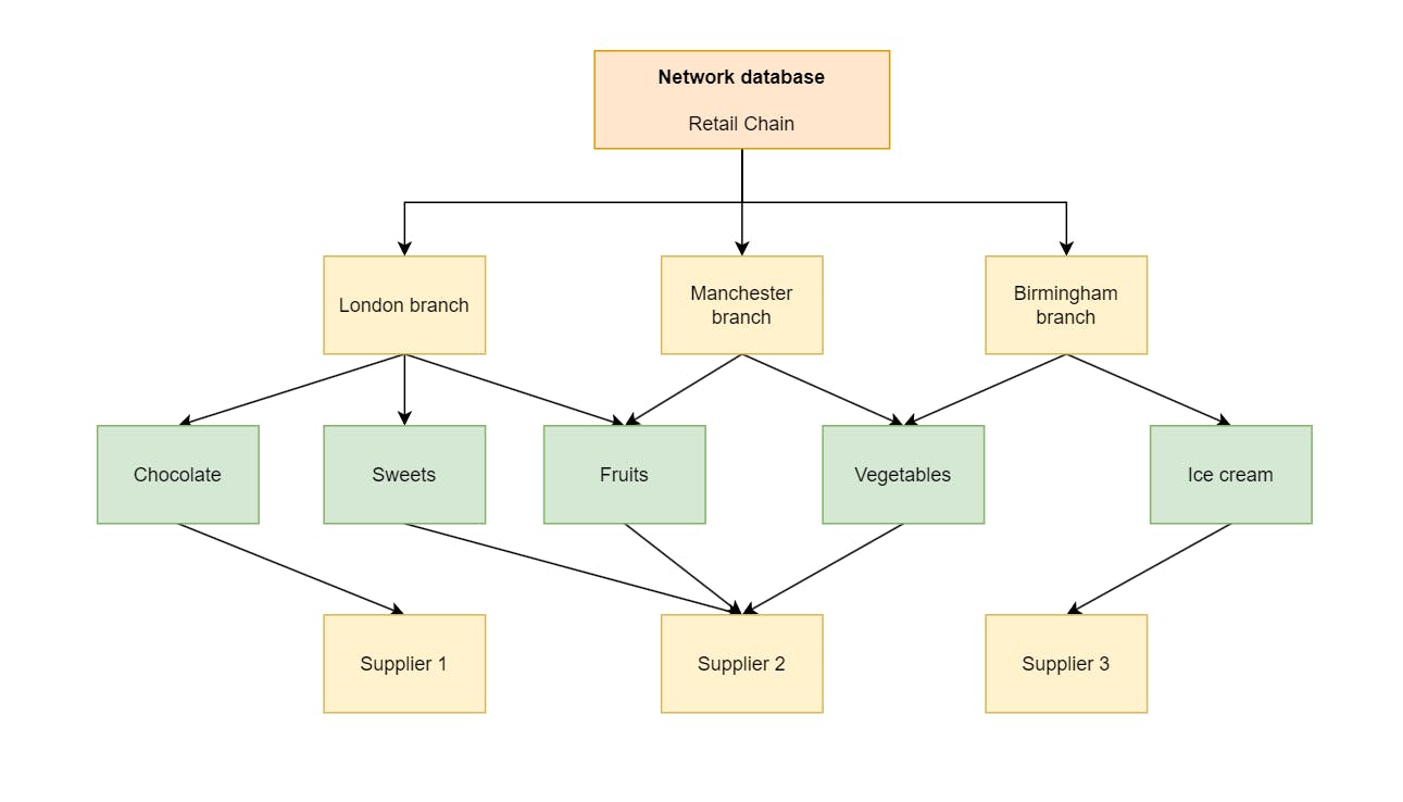
4. Network databases 🕸

These are also known as network data models, and they are similar to hierarchical databases. What distinguishes them from hierarchical databases is that any child node can have multiple parent nodes. This approach makes network databases organise data in a way that resembles a graph instead of a tree.

Hierarchical data models ran so that network data models could walk; as great as hierarchical data models were at data retrievals, network databases operated better at the same tasks due to the data modelling capabilities it introduced. Building one-to-one and one-to-many relationships is possible when you have multiple nodes that share similar attributes, which means more complex relationships could be built with them.

But there were problems with the network data model approach that couldn’t be ignored:

• Querying challenges ❓🔍- It is hard to query data under this type of database

• Maintenance issues 🛠️😖- Like the previous database, network data models are difficult to maintain as data sizes grow and more nodes are introduced into the complex architecture

So although you could build complex relationships using network databases, they were still more challenging to query and understand than their hierarchical counterpart.

After SQL⏩

Now with SQL, it is easier to access multiple records using a single line of code instead of manually searching yourself.

As a data engineer, SQL is a crucial language to have in your arsenal if you want to cover real-world data engineering use cases.

With SQL, we can

• analyse data

• retrieve data

• connect data

• manipulate data (update, delete, insert)

• build data models

Some of the different ways SQL is pronounced include:

• “Ess-cue-ell” (as if you’re spelling it out letter by letter as S-Q-L)

• “Se-quel” (as if you’re pronouncing the word sequel)

Let me know if you bump into any other variation of this too😄

Why SQL is the answer 💡

So how does SQL address the issues presented in the previous approaches?

• Standardized querying 📜✔️- The uniform language that SQL provides for interacting with data makes it one of its most popular attributes; there is a standard approach to collecting and shaping data no matter the difficulty level of your tasks.

• Easy & quick data retrieval⚡📂 - A SQL database can grant you immediate access to the data you require through techniques like indexing, where your data is stored into specific chunks that enable to SQL engine to retrieve them from the right places easily within milliseconds. This is a more efficient approach than sifting through several filing cabinets for a handful of records which could take hours, if not days in some cases.

• Flexible data modelling capabilities 🔗📊 - With SQL you can establish relationships between different tables by enforcing schemas, primary keys, data types and other constraints. Relationships can range from one-to-many, one-to-many, to many-to-many; SQL can support many complex relationships flexibly. This addresses some of the data integrity and quality concerns that are prevalent when using flat files as data stores.

• Data normalization 🔄📑- This technique ensures data is only stored once to avoid redundant data from entering the SQL database, therefore reducing inconsistencies and duplicates appearing in the tables.

• Simple maintenance 🛠️⏳- SQL databases were designed to scale even will relatively large data sizes and complex data relationships. The in-built algorithms managing the SQL engine’s operational backend make maintaining data easy over time with SQL, from automated backups to performance tuning.

• Advanced querying capabilities🔍⬆️ - Real-world data is complex, and SQL is purpose-built for it. If you want to join different tables together, filter data based on a list of complex criteria, or add conditional statements to columns, SQL can handle them all, among others.

Objects in SQL

Here are some of the objects you can create using SQL:

• databases

• schema

• tables

Database

This is the main object where the data is structured and organised for easy access and retrieval. It contains tables, views and indexes among other data objects useful for data analysis and manipulation. A typical SQL database is organised into tabular tables.

• Relational database - a type of database that organises data into structured tables. These tables contain primary keys, foreign keys and other integrity constraints to enable different tables to be connected to form more robust ones for data analysis. A relational database management system (RBDMS) is software that allows users to interact with relational databases, like SQL Server, PostgreSQL, and Oracle, among others.

• Non-relational databases - a type of database that stores data in non-structured collections. These databases do not require data to be structured in any specific format or defined schemas, which makes them useful for storing non-structured data. Technologies that support this include MongoDB, Cassandra, Neo4j

Schema

A schema is a container for a database’s tables, indexes, stored procedures and other data objects to reside in. Each database can have multiple schemas, but each schema can only reside in one database.

Table

A table is a collection of rows and columns that sit within the database. With tables, you can store different data types, like integers, strings, and dates, among others. Tables are primarily stored in relational databases.

Type of SQL commands

SQL commands are used to interact with the database for different purposes. Some of these purposes include creating databases, extracting data from specific columns, and managing access permissions, among many others. Here are the types of SQL commands:

• DDL - Data Definition Language

• DQL - Data Query Language

• DML - Data Manipulation Language

• DCL - Data Control Language

• TCL - Transaction Control Language

DDL (Data Definition Language)

These SQL commands are used to define the structure of a database, schema and/or table within the SQL server. The word define here includes any activity responsible for generating, changing or deleting the data objects mentioned and any items linked to them, thus the following commands:

• CREATE

• ALTER

• DROP

• RENAME

• TRUNCATE

• COMMENT

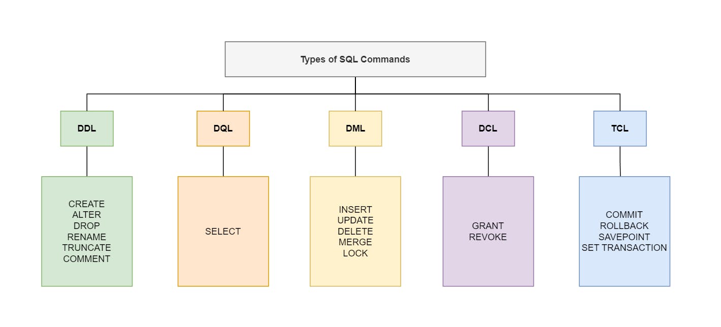
DQL (Data Query Language)

These commands are used to retrieve data from the database. The most popular one used is the SELECT statement.

DML (Data Manipulation Language)

These SQL commands can be used to manipulate the data within the databases or tables. The word manipulate can include any activity that involves inserting, updating or deleting data from the data objects, thus the following commands:

• INSERT

• UPDATE

• DELETE

• MERGE

• LOCK

DCL (Data Control Language)

These SQL commands are used to manage access to the databases. Commands for this include:

• GRANT

• REVOKE

TCL (Transaction Control Language)

These commands are used to manage the transactions in the database. In SQL, a transaction is a single unit of work that represents multiple operations for handling data integrity. The concept for this is tied to ACID transactions, which stand for:

• Atomicity💥- all operations within a single transaction either succeed together or fail together

• Consistency🔄 - the state of the database is the same before and after the transaction occurs

• Isolation🕴🏽 - Each transaction can run concurrently without interfering with each other

• Durability🔐- The changes made by the transaction are permanent

The SQL commands for this include:

• COMMIT

• ROLLBACK

• SAVEPOINT

• SET TRANSACTION

Basic SQL operations

• SELECT

• DISTINCT

• JOINS

• WHERE

• ORDER BY

SELECT

The SELECT statement is used to retrieve data from a SQL database. Here’s an example of how it can be used:

SELECT * FROM test_table;

This returns all the records from the test_table table.

DISTINCT

The DISTINCT statement is used to retrieve all the unique records in a specific column

SELECT DISTINCT column_1, column_2 
FROM test_table;

This returns all the unique records from the test_table table.

JOINS

A JOIN statement is used to connect more than one table through a common column. There are different types of JOIN statements, which include:

• INNER JOIN - Returns rows that contain matching values in both tables

• LEFT (OUTER) JOIN - Returns all the rows from the left table and the matching rows from the right table

• RIGHT (OUTER) JOIN - Returns all the rows from the right table and the matching rows from the left table

• FULL (OUTER) JOIN - Returns all the rows when there is a match found either in the left or right table

Here’s an example of an INNER JOIN:

SELECT a.column_1, b.column_2 
FROM test_table_1 a
INNER JOIN test_table_2 b 
ON a.common_column = b.common_column;

WHERE

A WHERE statement is used to filter the data by a certain condition:

SELECT * 
FROM test_table
WHERE column_1 > 20

This will only display data that contains values over 20 within column_1.

ORDER BY

An ORDER BY statement sorts the data based on at least one column in ascending or descending order:

SELECT * 
FROM test_table
ORDER BY 3 DESC

This will order the data by the 3rd column in descending order.